Cauchy
[3]:
# Parameters
func_name = "Cauchy"
positive_prior = False
Description
[5]:
func.display()
- description: The Cauchy distribution
- formula: $K\frac{1}{\gamma\pi}\left[\frac{\gamma^2}{(x-x_0)^2+\gamma^2}\right]$
- parameters:
- K:
- value: 1.0
- desc: Integral between -inf and +inf. Fix this to 1 to obtain a Cauchy distribution
- min_value: None
- max_value: None
- unit:
- is_normalization: False
- delta: 0.1
- free: True
- x0:
- value: 0.0
- desc: Central value
- min_value: None
- max_value: None
- unit:
- is_normalization: False
- delta: 0.1
- free: True
- gamma:
- value: 1.0
- desc: standard deviation
- min_value: 1e-12
- max_value: None
- unit:
- is_normalization: False
- delta: 0.1
- free: True
- K:
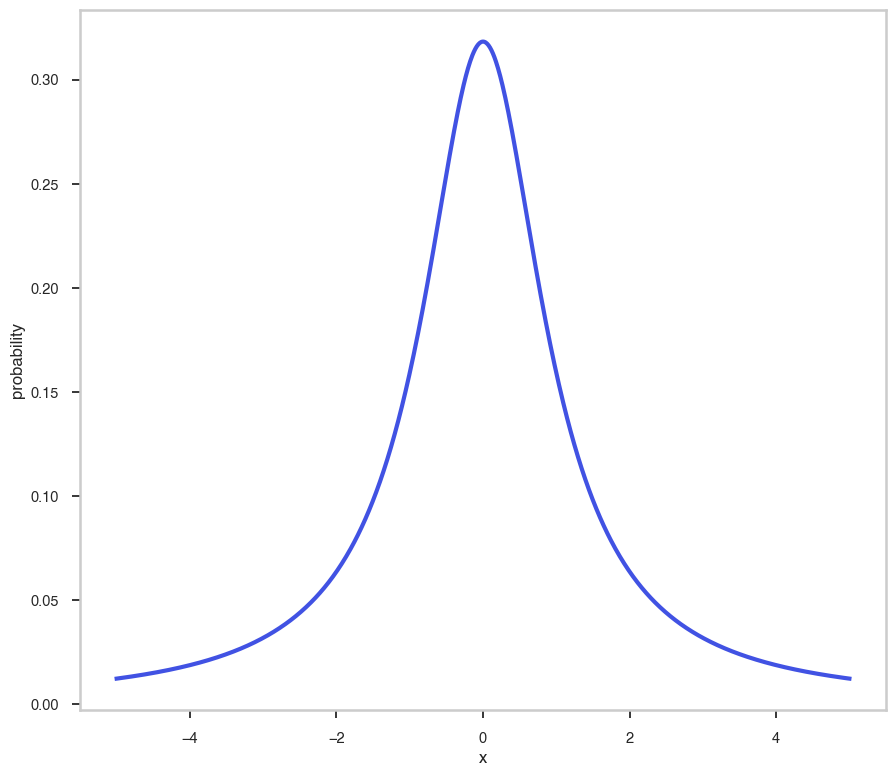
Shape
The shape of the function.
If this is not a photon model but a prior or linear function then ignore the units as these docs are auto-generated
[6]:
fig, ax = plt.subplots()


ax.plot(energy_grid, func(energy_grid), color=blue, lw=3)

ax.set_xlabel("x")
ax.set_ylabel("probability")
[6]:
Text(0, 0.5, 'probability')
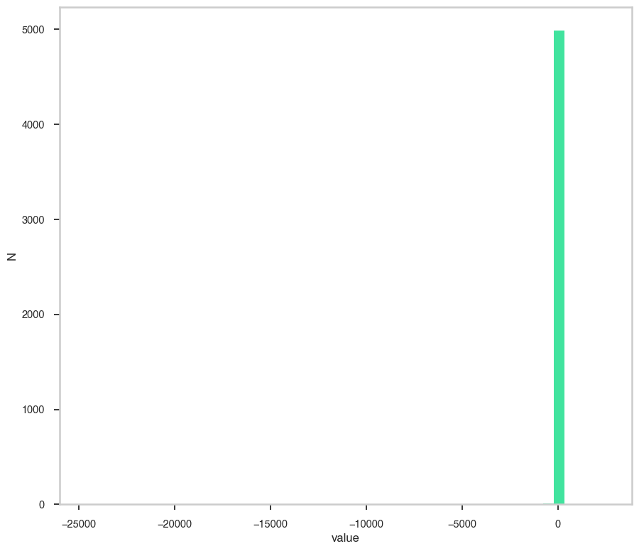
Random Number Generation
This is how we can generate random numbers from the prior.
[7]:
u = np.random.uniform(0,1, size=5000)

draws = [func.from_unit_cube(x) for x in u]


fig, ax = plt.subplots()


ax.hist(draws, color=green, bins=50)

ax.set_xlabel("value")
ax.set_ylabel("N")
[7]:
Text(0, 0.5, 'N')