Quick start
In this quick tutorial we will learn how to create a simple model with one point source, with a power law spectrum. You can of course use any function instead of the power law. Use list_models() to obtain a list of available models.
Let’s define the model:
[1]:
%%capture
from astromodels import *
[2]:
test_source = PointSource('test_source',ra=123.22, dec=-13.56, spectral_shape=Powerlaw_flux())

my_model = Model(test_source)
Now let’s use it:
[3]:
# Get and print the differential flux at 1 keV:

differential_flux_at_1_keV = my_model.test_source(1.0)

print("Differential flux @ 1 keV : %.3f photons / ( cm2 s keV)" % differential_flux_at_1_keV)
Differential flux @ 1 keV : 1.010 photons / ( cm2 s keV)
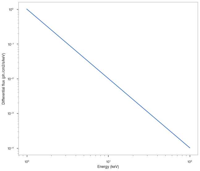
Evaluate the model on an array of 100 energies logarithmically distributed between 1 and 100 keV and plot it
[4]:
import numpy as np
import matplotlib.pyplot as plt
%matplotlib inline
from jupyterthemes import jtplot
jtplot.style(context="talk", fscale=1, ticks=True, grid=False)

# Set up the energies

energies = np.logspace(0,2,100)

# Get the differential flux

differential_flux = my_model.test_source(energies)


fig, ax = plt.subplots()

ax.loglog(energies, differential_flux)

ax.set_xlabel("Energy (keV)")
ax.set_ylabel("Differential flux (ph./cm2/s/keV)")
[4]:
Text(0, 0.5, 'Differential flux (ph./cm2/s/keV)')