Model tutorial
In this tutorial we show how to build a simple model with two point sources, how to save it for later use, and re-load it back. We will also plot the spectra of the two point sources, with their components.
See the documents about creating and getting information about functions, point sources and extended sources for details about these operations. Here we only focus on the global model.
[1]:
%%capture
from astromodels import *

# We also import astropy units to show the unit-conversion
# feature
import astropy.units as u
Define sources
Now let’s define a point source (see “Creating point sources” for details and alternative way to accomplish this):
[2]:
# Let's start by defining a simple point source with a power law spectrum
powerlaw = Powerlaw()

pts1 = PointSource('source_1', ra=125.6, dec=-75.3,
                   spectral_shape=powerlaw)

# Get some info about what we just created
pts1.display()
_setup
index
piv
K
_ipython_canary_method_should_not_exist_
_ipython_display_
_ipython_canary_method_should_not_exist_
_repr_mimebundle_
ra
dec
_ipython_canary_method_should_not_exist_
ra
dec
_ipython_canary_method_should_not_exist_
_repr_markdown_
_ipython_canary_method_should_not_exist_
_repr_svg_
_ipython_canary_method_should_not_exist_
_repr_png_
_ipython_canary_method_should_not_exist_
_repr_pdf_
_ipython_canary_method_should_not_exist_
_repr_jpeg_
_ipython_canary_method_should_not_exist_
_repr_latex_
_ipython_canary_method_should_not_exist_
_repr_json_
_ipython_canary_method_should_not_exist_
_repr_javascript_
- source_1 (point source):
- position:
- ra:
- value: 125.6
- desc: Right Ascension
- min_value: 0.0
- max_value: 360.0
- unit: deg
- is_normalization: False
- dec:
- value: -75.3
- desc: Declination
- min_value: -90.0
- max_value: 90.0
- unit: deg
- is_normalization: False
- equinox: J2000
- ra:
- spectrum:
- main:
- Powerlaw:
- K:
- value: 1.0
- desc: Normalization (differential flux at the pivot value)
- min_value: 1e-30
- max_value: 1000.0
- unit: keV-1 s-1 cm-2
- is_normalization: True
- piv:
- value: 1.0
- desc: Pivot value
- min_value: None
- max_value: None
- unit: keV
- is_normalization: False
- index:
- value: -2.01
- desc: Photon index
- min_value: -10.0
- max_value: 10.0
- unit:
- is_normalization: False
- K:
- Powerlaw:
- main:
- position:
Now let’s define another source, this time at Galactic Coordinates l = 11.25, b = -22.5, and with two spectral components:
[3]:
# Another point source with two spectral components

spectrum1 = Powerlaw(K=0.2, index=-0.75)
component1 = SpectralComponent('synchrotron',spectrum1)

spectrum2 = Powerlaw(K=0.8, index=-1.0)
component2 = SpectralComponent('IC',spectrum2)

point_source2 = PointSource('source_2', l=11.25, b=-22.5, components=[component1,component2])

# Have a look at what we just created

point_source2.display()
_setup
_setup
index
piv
K
index
piv
K
_ipython_canary_method_should_not_exist_
_ipython_display_
_ipython_canary_method_should_not_exist_
_repr_mimebundle_
l
b
_ipython_canary_method_should_not_exist_
l
b
_ipython_canary_method_should_not_exist_
_repr_markdown_
_ipython_canary_method_should_not_exist_
_repr_svg_
_ipython_canary_method_should_not_exist_
_repr_png_
_ipython_canary_method_should_not_exist_
_repr_pdf_
_ipython_canary_method_should_not_exist_
_repr_jpeg_
_ipython_canary_method_should_not_exist_
_repr_latex_
_ipython_canary_method_should_not_exist_
_repr_json_
_ipython_canary_method_should_not_exist_
_repr_javascript_
- source_2 (point source):
- position:
- l:
- value: 11.25
- desc: Galactic longitude
- min_value: 0.0
- max_value: 360.0
- unit: deg
- is_normalization: False
- b:
- value: -22.5
- desc: Galactic latitude
- min_value: -90.0
- max_value: 90.0
- unit: deg
- is_normalization: False
- equinox: J2000
- l:
- spectrum:
- synchrotron:
- Powerlaw:
- K:
- value: 0.20000000000000004
- desc: Normalization (differential flux at the pivot value)
- min_value: 1e-30
- max_value: 1000.0
- unit: keV-1 s-1 cm-2
- is_normalization: True
- piv:
- value: 1.0
- desc: Pivot value
- min_value: None
- max_value: None
- unit: keV
- is_normalization: False
- index:
- value: -0.75
- desc: Photon index
- min_value: -10.0
- max_value: 10.0
- unit:
- is_normalization: False
- K:
- Powerlaw:
- IC:
- Powerlaw:
- K:
- value: 0.8
- desc: Normalization (differential flux at the pivot value)
- min_value: 1e-30
- max_value: 1000.0
- unit: keV-1 s-1 cm-2
- is_normalization: True
- piv:
- value: 1.0
- desc: Pivot value
- min_value: None
- max_value: None
- unit: keV
- is_normalization: False
- index:
- value: -1.0
- desc: Photon index
- min_value: -10.0
- max_value: 10.0
- unit:
- is_normalization: False
- K:
- Powerlaw:
- synchrotron:
- position:
Create a model
Now let’s create our model, which comprises our two sources:
[4]:
# Build a model with the two point sources

my_model = Model(pts1, point_source2)
Of course you can use as many sources as needed, like my_model = Model(pts1, pts2, pts3…)
Getting information about a model
Using the .display() method we can see all free parameters currently in the model:
[5]:
my_model.display()
_ipython_canary_method_should_not_exist_
_ipython_display_
_ipython_canary_method_should_not_exist_
_repr_mimebundle_
spectrum
spectrum
spectrum
spectrum
_ipython_canary_method_should_not_exist_
spectrum
spectrum
spectrum
spectrum
_ipython_canary_method_should_not_exist_
_repr_markdown_
_ipython_canary_method_should_not_exist_
_repr_svg_
_ipython_canary_method_should_not_exist_
_repr_png_
_ipython_canary_method_should_not_exist_
_repr_pdf_
_ipython_canary_method_should_not_exist_
_repr_jpeg_
_ipython_canary_method_should_not_exist_
_repr_latex_
_ipython_canary_method_should_not_exist_
_repr_json_
_ipython_canary_method_should_not_exist_
_repr_javascript_
| N | |
|---|---|
| Point sources | 2 |
| Extended sources | 0 |
| Particle sources | 0 |
Free parameters (6):
| value | min_value | max_value | unit | |
|---|---|---|---|---|
| source_1.spectrum.main.Powerlaw.K | 1.0 | 0.0 | 1000.0 | keV-1 s-1 cm-2 |
| source_1.spectrum.main.Powerlaw.index | -2.01 | -10.0 | 10.0 | |
| source_2.spectrum.synchrotron.Powerlaw.K | 0.2 | 0.0 | 1000.0 | keV-1 s-1 cm-2 |
| source_2.spectrum.synchrotron.Powerlaw.index | -0.75 | -10.0 | 10.0 | |
| source_2.spectrum.IC.Powerlaw.K | 0.8 | 0.0 | 1000.0 | keV-1 s-1 cm-2 |
| source_2.spectrum.IC.Powerlaw.index | -1.0 | -10.0 | 10.0 |
Fixed parameters (7):
(abridged. Use complete=True to see all fixed parameters)
Properties (0):
(none)
Linked parameters (0):
(none)
Independent variables:
(none)
Linked functions (0):
(none)
A dictionary of free parameters can be obtained like this:
[6]:
free_parameters = my_model.free_parameters
We can use such dictionary to loop over all free parameters:
[7]:
for parameter_name, parameter in free_parameters.items():

    print("Parameter %s is free" % parameter_name)
Parameter source_1.spectrum.main.Powerlaw.K is free
Parameter source_1.spectrum.main.Powerlaw.index is free
Parameter source_2.spectrum.synchrotron.Powerlaw.K is free
Parameter source_2.spectrum.synchrotron.Powerlaw.index is free
Parameter source_2.spectrum.IC.Powerlaw.K is free
Parameter source_2.spectrum.IC.Powerlaw.index is free
More information on a particular source can be obtained like:
[8]:
my_model.source_1.display()
source_1
_ipython_canary_method_should_not_exist_
_ipython_display_
_ipython_canary_method_should_not_exist_
_repr_mimebundle_
ra
dec
_ipython_canary_method_should_not_exist_
ra
dec
_ipython_canary_method_should_not_exist_
_repr_markdown_
_ipython_canary_method_should_not_exist_
_repr_svg_
_ipython_canary_method_should_not_exist_
_repr_png_
_ipython_canary_method_should_not_exist_
_repr_pdf_
_ipython_canary_method_should_not_exist_
_repr_jpeg_
_ipython_canary_method_should_not_exist_
_repr_latex_
_ipython_canary_method_should_not_exist_
_repr_json_
_ipython_canary_method_should_not_exist_
_repr_javascript_
- source_1 (point source):
- position:
- ra:
- value: 125.6
- desc: Right Ascension
- min_value: 0.0
- max_value: 360.0
- unit: deg
- is_normalization: False
- dec:
- value: -75.3
- desc: Declination
- min_value: -90.0
- max_value: 90.0
- unit: deg
- is_normalization: False
- equinox: J2000
- ra:
- spectrum:
- main:
- Powerlaw:
- K:
- value: 1.0
- desc: Normalization (differential flux at the pivot value)
- min_value: 1e-30
- max_value: 1000.0
- unit: keV-1 s-1 cm-2
- is_normalization: True
- piv:
- value: 1.0
- desc: Pivot value
- min_value: None
- max_value: None
- unit: keV
- is_normalization: False
- index:
- value: -2.01
- desc: Photon index
- min_value: -10.0
- max_value: 10.0
- unit:
- is_normalization: False
- K:
- Powerlaw:
- main:
- position:
More information about a particular instance of a function can be obtained like:
[9]:
my_model.source_1.spectrum.main.Powerlaw.display()
source_1
spectrum
main
Powerlaw
_ipython_canary_method_should_not_exist_
_ipython_display_
_ipython_canary_method_should_not_exist_
_repr_mimebundle_
_ipython_canary_method_should_not_exist_
_ipython_canary_method_should_not_exist_
_repr_markdown_
_ipython_canary_method_should_not_exist_
_repr_svg_
_ipython_canary_method_should_not_exist_
_repr_png_
_ipython_canary_method_should_not_exist_
_repr_pdf_
_ipython_canary_method_should_not_exist_
_repr_jpeg_
_ipython_canary_method_should_not_exist_
_repr_latex_
_ipython_canary_method_should_not_exist_
_repr_json_
_ipython_canary_method_should_not_exist_
_repr_javascript_
- description: A simple power-law
- formula: $ K~\frac{x}{piv}^{index} $
- parameters:
- K:
- value: 1.0
- desc: Normalization (differential flux at the pivot value)
- min_value: 1e-30
- max_value: 1000.0
- unit: keV-1 s-1 cm-2
- is_normalization: True
- delta: 0.1
- free: True
- piv:
- value: 1.0
- desc: Pivot value
- min_value: None
- max_value: None
- unit: keV
- is_normalization: False
- delta: 0.1
- free: False
- index:
- value: -2.01
- desc: Photon index
- min_value: -10.0
- max_value: 10.0
- unit:
- is_normalization: False
- delta: 0.20099999999999998
- free: True
- K:
Accessing and modifying sources and parameters from the model instance
Fully-qualified paths
Each source and each parameter has a precise path within the model. These paths are displayed by the .display() method of the model instance (see above), and can be used like my_model.[path]. For example:
[10]:
my_model.display()
_ipython_canary_method_should_not_exist_
_ipython_display_
_ipython_canary_method_should_not_exist_
_repr_mimebundle_
spectrum
spectrum
spectrum
spectrum
_ipython_canary_method_should_not_exist_
spectrum
spectrum
spectrum
spectrum
_ipython_canary_method_should_not_exist_
_repr_markdown_
_ipython_canary_method_should_not_exist_
_repr_svg_
_ipython_canary_method_should_not_exist_
_repr_png_
_ipython_canary_method_should_not_exist_
_repr_pdf_
_ipython_canary_method_should_not_exist_
_repr_jpeg_
_ipython_canary_method_should_not_exist_
_repr_latex_
_ipython_canary_method_should_not_exist_
_repr_json_
_ipython_canary_method_should_not_exist_
_repr_javascript_
| N | |
|---|---|
| Point sources | 2 |
| Extended sources | 0 |
| Particle sources | 0 |
Free parameters (6):
| value | min_value | max_value | unit | |
|---|---|---|---|---|
| source_1.spectrum.main.Powerlaw.K | 1.0 | 0.0 | 1000.0 | keV-1 s-1 cm-2 |
| source_1.spectrum.main.Powerlaw.index | -2.01 | -10.0 | 10.0 | |
| source_2.spectrum.synchrotron.Powerlaw.K | 0.2 | 0.0 | 1000.0 | keV-1 s-1 cm-2 |
| source_2.spectrum.synchrotron.Powerlaw.index | -0.75 | -10.0 | 10.0 | |
| source_2.spectrum.IC.Powerlaw.K | 0.8 | 0.0 | 1000.0 | keV-1 s-1 cm-2 |
| source_2.spectrum.IC.Powerlaw.index | -1.0 | -10.0 | 10.0 |
Fixed parameters (7):
(abridged. Use complete=True to see all fixed parameters)
Properties (0):
(none)
Linked parameters (0):
(none)
Independent variables:
(none)
Linked functions (0):
(none)
[11]:
# Access the logK parameters of the powerlaw spectrum of the main component for source 1:

my_model.source_1.spectrum.main.Powerlaw.logK = -0.5

# Access the logK parameters of the spectrum of the IC component of source 2:

my_model.source_2.spectrum.IC.Powerlaw.logK = -0.32
source_1
spectrum
main
Powerlaw
source_2
spectrum
IC
Powerlaw
The structure of these paths is easy to understand. The model is a tree-like structure. The root of the tree is always the model instance itself. The second level is constituted by the various sources. The structure within a source can be understood by calling the .display method:
[12]:
my_model.source_1.display()
source_1
_ipython_canary_method_should_not_exist_
_ipython_display_
_ipython_canary_method_should_not_exist_
_repr_mimebundle_
ra
dec
_ipython_canary_method_should_not_exist_
ra
dec
_ipython_canary_method_should_not_exist_
_repr_markdown_
_ipython_canary_method_should_not_exist_
_repr_svg_
_ipython_canary_method_should_not_exist_
_repr_png_
_ipython_canary_method_should_not_exist_
_repr_pdf_
_ipython_canary_method_should_not_exist_
_repr_jpeg_
_ipython_canary_method_should_not_exist_
_repr_latex_
_ipython_canary_method_should_not_exist_
_repr_json_
_ipython_canary_method_should_not_exist_
_repr_javascript_
- source_1 (point source):
- position:
- ra:
- value: 125.6
- desc: Right Ascension
- min_value: 0.0
- max_value: 360.0
- unit: deg
- is_normalization: False
- dec:
- value: -75.3
- desc: Declination
- min_value: -90.0
- max_value: 90.0
- unit: deg
- is_normalization: False
- equinox: J2000
- ra:
- spectrum:
- main:
- Powerlaw:
- K:
- value: 1.0
- desc: Normalization (differential flux at the pivot value)
- min_value: 1e-30
- max_value: 1000.0
- unit: keV-1 s-1 cm-2
- is_normalization: True
- piv:
- value: 1.0
- desc: Pivot value
- min_value: None
- max_value: None
- unit: keV
- is_normalization: False
- index:
- value: -2.01
- desc: Photon index
- min_value: -10.0
- max_value: 10.0
- unit:
- is_normalization: False
- K:
- Powerlaw:
- main:
- position:
Each indentation represents one level, so to access the “ra” element we can follow the levels shown by the .display() method:
[13]:
ra_parameter = my_model.source_1.position.ra

ra_parameter.display()
source_1
position
ra
_ipython_canary_method_should_not_exist_
_ipython_display_
_ipython_canary_method_should_not_exist_
_repr_mimebundle_
_ipython_canary_method_should_not_exist_
_ipython_canary_method_should_not_exist_
_repr_markdown_
_ipython_canary_method_should_not_exist_
_repr_svg_
_ipython_canary_method_should_not_exist_
_repr_png_
_ipython_canary_method_should_not_exist_
_repr_pdf_
_ipython_canary_method_should_not_exist_
_repr_jpeg_
_ipython_canary_method_should_not_exist_
_repr_latex_
_ipython_canary_method_should_not_exist_
_repr_json_
_ipython_canary_method_should_not_exist_
_repr_javascript_
Note: this is a Parameter instance. To get the position of the source as a floating point number, use: my_model.source_1.position.get_ra() which will work for any source
while to access the index parameter of the power law function we can do
[14]:
K_parameter = my_model.source_1.spectrum.main.Powerlaw.K

K_parameter.display()
source_1
spectrum
main
Powerlaw
K
_ipython_canary_method_should_not_exist_
_ipython_display_
_ipython_canary_method_should_not_exist_
_repr_mimebundle_
_ipython_canary_method_should_not_exist_
_ipython_canary_method_should_not_exist_
_repr_markdown_
_ipython_canary_method_should_not_exist_
_repr_svg_
_ipython_canary_method_should_not_exist_
_repr_png_
_ipython_canary_method_should_not_exist_
_repr_pdf_
_ipython_canary_method_should_not_exist_
_repr_jpeg_
_ipython_canary_method_should_not_exist_
_repr_latex_
_ipython_canary_method_should_not_exist_
_repr_json_
_ipython_canary_method_should_not_exist_
_repr_javascript_
You can find much more information in the document “Additional features for scripts and applications”.
These fully-qualified paths are unique to each element, are very descriptive and easy to understand. They can always be used and are encouraged in general, but especially in scripts, when the effort spent writing them is paid off in terms of clarity. However, there is an alternative way which might be more convenient in certain situation, especially when models are simple and the chances of getting confused are low. This alternative method is described below.
Using shortcuts
Exploiting the feature of the python language, we can create names (“shortcuts”) for objects:
[15]:
# Create a "shortcut" for the spectrum of a source

powerlaw_1 = my_model.source_1.spectrum.main.Powerlaw

# Now we can change the values of that power law as:
powerlaw_1.K = 1.2

# GOTCHA: while it is possible to create shortcuts for parameters, it is not encouraged
# Indeed, this will not work:
# logK_1 = my_model.source_1.spectrum.main.powerlaw.logK
# logK_1 = -1.2 # WILL NOT WORK
# In order to use a shortcut for a parameter to change its value, you have to explicitly
# set its property 'value':
# logK_1.value = -1.2 # This will work
source_1
spectrum
main
Powerlaw
GOTACH: while it is possible to create shortcuts for parameters, it is not encouraged. Indeed, this will not work:
K_1 = my_model.source_1.spectrum.main.powerlaw.K
K_1 = 1.2 WILL NOT WORK
In order to use a shortcut for a parameter to change its value, you have to explicitly set its property ‘value’: K_1.value = 1.2 This will work
Shortcut can point at any point of the tree:
[16]:
# Create a shortcut of a source
source_1 = my_model.source_1

# Now we can do:
source_1.spectrum.main.Powerlaw.index = -2.3

# Create a shortcut for a component

main_component = my_model.source_1.spectrum.main

# Now we can do:
main_component.Powerlaw.index = -1.3
source_1
spectrum
main
Powerlaw
source_1
spectrum
main
Powerlaw
If you are ever in doubt of what a particular shortcut stands for, you can always retrieve the full path of the element the shortcut is pointing to like this:
[17]:
print(main_component.path)
source_1.spectrum.main
Saving a model to file
An existing model can be saved to a file with:
[18]:
# Save the model to a file, overwriting it if already existing

my_model.save('my_model.yml', overwrite=True)
ra
dec
l
b
The content of the file is YAML code, which is human-readable and very easy to understand. Let’s have a look:
[19]:
with open('my_model.yml') as yaml_file:

    print("".join(yaml_file.readlines()))
source_1 (point source):

  position:

    ra:

      value: 125.6

      desc: Right Ascension

      min_value: 0.0

      max_value: 360.0

      unit: deg

      is_normalization: false

      delta: 12.56

      free: false

    dec:

      value: -75.3

      desc: Declination

      min_value: -90.0

      max_value: 90.0

      unit: deg

      is_normalization: false

      delta: 7.53

      free: false

    equinox: J2000

  spectrum:

    main:

      Powerlaw:

        K:

          value: 1.2

          desc: Normalization (differential flux at the pivot value)

          min_value: 1.0e-30

          max_value: 1000.0

          unit: keV-1 s-1 cm-2

          is_normalization: true

          delta: 0.1

          free: true

        piv:

          value: 1.0

          desc: Pivot value

          min_value: null

          max_value: null

          unit: keV

          is_normalization: false

          delta: 0.1

          free: false

        index:

          value: -1.3

          desc: Photon index

          min_value: -10.0

          max_value: 10.0

          unit: ''

          is_normalization: false

          delta: 0.20099999999999998

          free: true

      polarization: {}

source_2 (point source):

  position:

    l:

      value: 11.25

      desc: Galactic longitude

      min_value: 0.0

      max_value: 360.0

      unit: deg

      is_normalization: false

      delta: 1.125

      free: false

    b:

      value: -22.5

      desc: Galactic latitude

      min_value: -90.0

      max_value: 90.0

      unit: deg

      is_normalization: false

      delta: 2.25

      free: false

    equinox: J2000

  spectrum:

    synchrotron:

      Powerlaw:

        K:

          value: 0.20000000000000004

          desc: Normalization (differential flux at the pivot value)

          min_value: 1.0e-30

          max_value: 1000.0

          unit: keV-1 s-1 cm-2

          is_normalization: true

          delta: 0.1

          free: true

        piv:

          value: 1.0

          desc: Pivot value

          min_value: null

          max_value: null

          unit: keV

          is_normalization: false

          delta: 0.1

          free: false

        index:

          value: -0.75

          desc: Photon index

          min_value: -10.0

          max_value: 10.0

          unit: ''

          is_normalization: false

          delta: 0.20099999999999998

          free: true

      polarization: {}

    IC:

      Powerlaw:

        K:

          value: 0.8

          desc: Normalization (differential flux at the pivot value)

          min_value: 1.0e-30

          max_value: 1000.0

          unit: keV-1 s-1 cm-2

          is_normalization: true

          delta: 0.1

          free: true

        piv:

          value: 1.0

          desc: Pivot value

          min_value: null

          max_value: null

          unit: keV

          is_normalization: false

          delta: 0.1

          free: false

        index:

          value: -1.0

          desc: Photon index

          min_value: -10.0

          max_value: 10.0

          unit: ''

          is_normalization: false

          delta: 0.20099999999999998

          free: true

      polarization: {}
Load a model from a file
Now suppose that you want to load back a file you created in a previous session. You can do it with:
[20]:
my_model = load_model('my_model.yml')

# Explore the model we just loaded back

my_model.display()
_setup
index
piv
K
_setup
_setup
index
piv
K
index
piv
K
_ipython_canary_method_should_not_exist_
_ipython_display_
_ipython_canary_method_should_not_exist_
_repr_mimebundle_
spectrum
spectrum
spectrum
spectrum
_ipython_canary_method_should_not_exist_
spectrum
spectrum
spectrum
spectrum
_ipython_canary_method_should_not_exist_
_repr_markdown_
_ipython_canary_method_should_not_exist_
_repr_svg_
_ipython_canary_method_should_not_exist_
_repr_png_
_ipython_canary_method_should_not_exist_
_repr_pdf_
_ipython_canary_method_should_not_exist_
_repr_jpeg_
_ipython_canary_method_should_not_exist_
_repr_latex_
_ipython_canary_method_should_not_exist_
_repr_json_
_ipython_canary_method_should_not_exist_
_repr_javascript_
| N | |
|---|---|
| Point sources | 2 |
| Extended sources | 0 |
| Particle sources | 0 |
Free parameters (6):
| value | min_value | max_value | unit | |
|---|---|---|---|---|
| source_1.spectrum.main.Powerlaw.K | 1.2 | 0.0 | 1000.0 | keV-1 s-1 cm-2 |
| source_1.spectrum.main.Powerlaw.index | -1.3 | -10.0 | 10.0 | |
| source_2.spectrum.synchrotron.Powerlaw.K | 0.2 | 0.0 | 1000.0 | keV-1 s-1 cm-2 |
| source_2.spectrum.synchrotron.Powerlaw.index | -0.75 | -10.0 | 10.0 | |
| source_2.spectrum.IC.Powerlaw.K | 0.8 | 0.0 | 1000.0 | keV-1 s-1 cm-2 |
| source_2.spectrum.IC.Powerlaw.index | -1.0 | -10.0 | 10.0 |
Fixed parameters (7):
(abridged. Use complete=True to see all fixed parameters)
Properties (0):
(none)
Linked parameters (0):
(none)
Independent variables:
(none)
Linked functions (0):
(none)
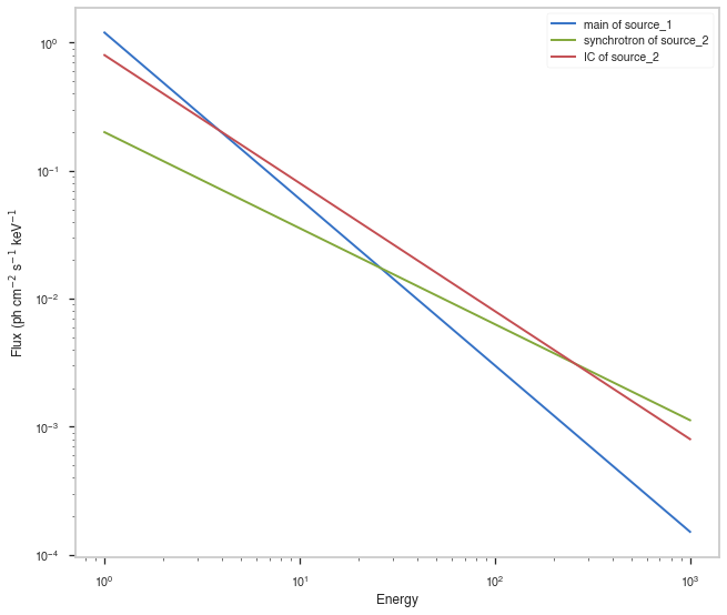
[21]:
# Now evaluate and plot our models. You need matplotlib for this

import numpy as np
import matplotlib.pyplot as plt
%matplotlib inline
from jupyterthemes import jtplot
jtplot.style(context="talk", fscale=1, ticks=True, grid=False)


fig, ax = plt.subplots()
# Energies where we want to evaluate the model

e = np.geomspace(1,1000,100)

# Loop over the sources

for src_name, src in my_model.point_sources.items():

    # Loop over the components of each source

    for comp_name, component in src.components.items():

        # Get the differential flux (in ph/cm2/s)

        flux = component.shape(e)

        # this can also be accomplished with:
        # flux = component.powerlaw(e)
        # but this requires to know the name of the
        # spectral shape which was used

        # Plot this component for this source

        ax.loglog(e, flux,label="%s of %s" % (component.name, src.name))

ax.legend(loc=0)

ax.set_xlabel("Energy")
ax.set_ylabel(r"Flux (ph cm$^{-2}$ s$^{-1}$ keV$^{-1}$")
[21]:
Text(0, 0.5, 'Flux (ph cm$^{-2}$ s$^{-1}$ keV$^{-1}$')
Linking parameters
Sometimes you want to link two parameters of a model so that they have the same value. This can be easily accomplished in astromodels:
[22]:
# Link the photon index of the first source with the
# photon index of the IC component of the second source

my_model.link(my_model.source_2.spectrum.IC.Powerlaw.index,
              my_model.source_1.spectrum.main.Powerlaw.index)

my_model.display()
source_2
spectrum
IC
Powerlaw
index
source_1
spectrum
main
Powerlaw
index
_setup
a
a
b
b
a
b
a
b
_ipython_canary_method_should_not_exist_
_ipython_display_
_ipython_canary_method_should_not_exist_
_repr_mimebundle_
spectrum
spectrum
spectrum
spectrum
_ipython_canary_method_should_not_exist_
spectrum
spectrum
spectrum
spectrum
_ipython_canary_method_should_not_exist_
_repr_markdown_
_ipython_canary_method_should_not_exist_
_repr_svg_
_ipython_canary_method_should_not_exist_
_repr_png_
_ipython_canary_method_should_not_exist_
_repr_pdf_
_ipython_canary_method_should_not_exist_
_repr_jpeg_
_ipython_canary_method_should_not_exist_
_repr_latex_
_ipython_canary_method_should_not_exist_
_repr_json_
_ipython_canary_method_should_not_exist_
_repr_javascript_
| N | |
|---|---|
| Point sources | 2 |
| Extended sources | 0 |
| Particle sources | 0 |
Free parameters (5):
| value | min_value | max_value | unit | |
|---|---|---|---|---|
| source_1.spectrum.main.Powerlaw.K | 1.2 | 0.0 | 1000.0 | keV-1 s-1 cm-2 |
| source_1.spectrum.main.Powerlaw.index | -1.3 | -10.0 | 10.0 | |
| source_2.spectrum.synchrotron.Powerlaw.K | 0.2 | 0.0 | 1000.0 | keV-1 s-1 cm-2 |
| source_2.spectrum.synchrotron.Powerlaw.index | -0.75 | -10.0 | 10.0 | |
| source_2.spectrum.IC.Powerlaw.K | 0.8 | 0.0 | 1000.0 | keV-1 s-1 cm-2 |
Fixed parameters (9):
(abridged. Use complete=True to see all fixed parameters)
Properties (0):
(none)
Linked parameters (1):
| source_2.spectrum.IC.Powerlaw.index | |
|---|---|
| current value | -1.3 |
| function | Line |
| linked to | source_1.spectrum.main.Powerlaw.index |
| unit |
Independent variables:
(none)
Linked functions (0):
(none)
Advanced use of linking: arbitrary functions
Astromodels takes this a step further. Parameters can be linked to each other through any function. The parameters of the linking function become parameters of the model like any other, and can be left free to vary or fixed. For example, let’s consider the case where we want the photon index of the IC component of the second source (p2) to be equal to the photon index of the first source (p1) plus a constant. We can link the two parameters with the ‘bias’ function \(f(x) = x + k\), so that \(p2(p1) = p1 + k\):
[23]:
# Link the photon indexes through the 'linear' function, i.e.,
# the photon index of the IC component of the second source is fixed to be the
# photon index of the first source plus a constant k

link_function = Line(a=2, b=1)
link_function.b.fix=True

my_model.link(my_model.source_2.spectrum.IC.Powerlaw.index,
              my_model.source_1.spectrum.main.Powerlaw.index,
              link_function)

# The parameters of the linking function become parameters
# of the model, and are put in the model tree under the parameter they are
# linking.
# In this case the only parameter of the 'linear' function ('k') becomes then
# my_model.source_2.spectrum.IC.powerlaw.logK.bias.k

my_model.display()
_setup
b
source_2
spectrum
IC
Powerlaw
index
source_1
spectrum
main
Powerlaw
index
a
b
a
b
_ipython_canary_method_should_not_exist_
_ipython_display_
_ipython_canary_method_should_not_exist_
_repr_mimebundle_
spectrum
spectrum
spectrum
spectrum
_ipython_canary_method_should_not_exist_
spectrum
spectrum
spectrum
spectrum
_ipython_canary_method_should_not_exist_
_repr_markdown_
_ipython_canary_method_should_not_exist_
_repr_svg_
_ipython_canary_method_should_not_exist_
_repr_png_
_ipython_canary_method_should_not_exist_
_repr_pdf_
_ipython_canary_method_should_not_exist_
_repr_jpeg_
_ipython_canary_method_should_not_exist_
_repr_latex_
_ipython_canary_method_should_not_exist_
_repr_json_
_ipython_canary_method_should_not_exist_
_repr_javascript_
| N | |
|---|---|
| Point sources | 2 |
| Extended sources | 0 |
| Particle sources | 0 |
Free parameters (6):
| value | min_value | max_value | unit | |
|---|---|---|---|---|
| source_1.spectrum.main.Powerlaw.K | 1.2 | 0.0 | 1000.0 | keV-1 s-1 cm-2 |
| source_1.spectrum.main.Powerlaw.index | -1.3 | -10.0 | 10.0 | |
| source_2.spectrum.synchrotron.Powerlaw.K | 0.2 | 0.0 | 1000.0 | keV-1 s-1 cm-2 |
| source_2.spectrum.synchrotron.Powerlaw.index | -0.75 | -10.0 | 10.0 | |
| source_2.spectrum.IC.Powerlaw.K | 0.8 | 0.0 | 1000.0 | keV-1 s-1 cm-2 |
| source_2.spectrum.IC.Powerlaw.index.Line.a | 2.0 | None | None |
Fixed parameters (8):
(abridged. Use complete=True to see all fixed parameters)
Properties (0):
(none)
Linked parameters (1):
| source_2.spectrum.IC.Powerlaw.index | |
|---|---|
| current value | 0.7 |
| function | Line |
| linked to | source_1.spectrum.main.Powerlaw.index |
| unit |
Independent variables:
(none)
Linked functions (0):
(none)
If we want to fix say \(p2 = p1 - 1.2\), we can fix k to that:
[24]:
my_model.source_2.spectrum.IC.Powerlaw.index.Line.a = -1.2
my_model.source_2.spectrum.IC.Powerlaw.index.Line.a.fix = True

my_model.display()
source_2
spectrum
IC
Powerlaw
index
Line
source_2
spectrum
IC
Powerlaw
index
Line
a
_ipython_canary_method_should_not_exist_
_ipython_display_
_ipython_canary_method_should_not_exist_
_repr_mimebundle_
spectrum
spectrum
spectrum
spectrum
_ipython_canary_method_should_not_exist_
spectrum
spectrum
spectrum
spectrum
_ipython_canary_method_should_not_exist_
_repr_markdown_
_ipython_canary_method_should_not_exist_
_repr_svg_
_ipython_canary_method_should_not_exist_
_repr_png_
_ipython_canary_method_should_not_exist_
_repr_pdf_
_ipython_canary_method_should_not_exist_
_repr_jpeg_
_ipython_canary_method_should_not_exist_
_repr_latex_
_ipython_canary_method_should_not_exist_
_repr_json_
_ipython_canary_method_should_not_exist_
_repr_javascript_
| N | |
|---|---|
| Point sources | 2 |
| Extended sources | 0 |
| Particle sources | 0 |
Free parameters (5):
| value | min_value | max_value | unit | |
|---|---|---|---|---|
| source_1.spectrum.main.Powerlaw.K | 1.2 | 0.0 | 1000.0 | keV-1 s-1 cm-2 |
| source_1.spectrum.main.Powerlaw.index | -1.3 | -10.0 | 10.0 | |
| source_2.spectrum.synchrotron.Powerlaw.K | 0.2 | 0.0 | 1000.0 | keV-1 s-1 cm-2 |
| source_2.spectrum.synchrotron.Powerlaw.index | -0.75 | -10.0 | 10.0 | |
| source_2.spectrum.IC.Powerlaw.K | 0.8 | 0.0 | 1000.0 | keV-1 s-1 cm-2 |
Fixed parameters (9):
(abridged. Use complete=True to see all fixed parameters)
Properties (0):
(none)
Linked parameters (1):
| source_2.spectrum.IC.Powerlaw.index | |
|---|---|
| current value | -2.5 |
| function | Line |
| linked to | source_1.spectrum.main.Powerlaw.index |
| unit |
Independent variables:
(none)
Linked functions (0):
(none)
As another example, we might link the two parameters using a power law function:
[25]:
my_model.link(my_model.source_2.spectrum.IC.Powerlaw.index,
              my_model.source_1.spectrum.main.Powerlaw.index,
              Powerlaw())

my_model.display()
source_2
spectrum
IC
Powerlaw
index
source_1
spectrum
main
Powerlaw
index
_setup
index
piv
K
index
piv
K
_ipython_canary_method_should_not_exist_
_ipython_display_
_ipython_canary_method_should_not_exist_
_repr_mimebundle_
spectrum
spectrum
spectrum
spectrum
_ipython_canary_method_should_not_exist_
spectrum
spectrum
spectrum
spectrum
_ipython_canary_method_should_not_exist_
_repr_markdown_
_ipython_canary_method_should_not_exist_
_repr_svg_
_ipython_canary_method_should_not_exist_
_repr_png_
_ipython_canary_method_should_not_exist_
_repr_pdf_
_ipython_canary_method_should_not_exist_
_repr_jpeg_
_ipython_canary_method_should_not_exist_
_repr_latex_
_ipython_canary_method_should_not_exist_
_repr_json_
_ipython_canary_method_should_not_exist_
_repr_javascript_
| N | |
|---|---|
| Point sources | 2 |
| Extended sources | 0 |
| Particle sources | 0 |
Free parameters (7):
| value | min_value | max_value | unit | |
|---|---|---|---|---|
| source_1.spectrum.main.Powerlaw.K | 1.2 | 0.0 | 1000.0 | keV-1 s-1 cm-2 |
| source_1.spectrum.main.Powerlaw.index | -1.3 | -10.0 | 10.0 | |
| source_2.spectrum.synchrotron.Powerlaw.K | 0.2 | 0.0 | 1000.0 | keV-1 s-1 cm-2 |
| source_2.spectrum.synchrotron.Powerlaw.index | -0.75 | -10.0 | 10.0 | |
| source_2.spectrum.IC.Powerlaw.K | 0.8 | 0.0 | 1000.0 | keV-1 s-1 cm-2 |
| source_2.spectrum.IC.Powerlaw.index.Powerlaw.K | 1.0 | 0.0 | 1000.0 | |
| source_2.spectrum.IC.Powerlaw.index.Powerlaw.index | -2.01 | -10.0 | 10.0 |
Fixed parameters (10):
(abridged. Use complete=True to see all fixed parameters)
Properties (0):
(none)
Linked parameters (1):
| source_2.spectrum.IC.Powerlaw.index | |
|---|---|
| current value | NaN |
| function | Powerlaw |
| linked to | source_1.spectrum.main.Powerlaw.index |
| unit |
Independent variables:
(none)
Linked functions (0):
(none)
We can use arbitrarily complex functions as link function, if needed (see “Creating and modifying functions” for more info on how to create composite functions):
[26]:
# A random composite function (see "Creating and modifying functions" for more info)
crazy_link = Powerlaw() + Gaussian()

my_model.link(my_model.source_2.spectrum.IC.Powerlaw.index,
              my_model.source_1.spectrum.main.Powerlaw.index,
              crazy_link)

my_model.display()
_setup
source_2
spectrum
IC
Powerlaw
index
source_1
spectrum
main
Powerlaw
index
_make_dimensionless
index
piv
K
_make_dimensionless
F
mu
sigma
_make_dimensionless
index
piv
K
_make_dimensionless
F
mu
sigma
_ipython_canary_method_should_not_exist_
_ipython_display_
_ipython_canary_method_should_not_exist_
_repr_mimebundle_
spectrum
spectrum
spectrum
spectrum
_ipython_canary_method_should_not_exist_
spectrum
spectrum
spectrum
spectrum
_ipython_canary_method_should_not_exist_
_repr_markdown_
_ipython_canary_method_should_not_exist_
_repr_svg_
_ipython_canary_method_should_not_exist_
_repr_png_
_ipython_canary_method_should_not_exist_
_repr_pdf_
_ipython_canary_method_should_not_exist_
_repr_jpeg_
_ipython_canary_method_should_not_exist_
_repr_latex_
_ipython_canary_method_should_not_exist_
_repr_json_
_ipython_canary_method_should_not_exist_
_repr_javascript_
| N | |
|---|---|
| Point sources | 2 |
| Extended sources | 0 |
| Particle sources | 0 |
Free parameters (12):
| value | min_value | max_value | unit | |
|---|---|---|---|---|
| source_1.spectrum.main.Powerlaw.K | 1.2 | 0.0 | 1000.0 | keV-1 s-1 cm-2 |
| source_1.spectrum.main.Powerlaw.index | -1.3 | -10.0 | 10.0 | |
| source_2.spectrum.synchrotron.Powerlaw.K | 0.2 | 0.0 | 1000.0 | keV-1 s-1 cm-2 |
| source_2.spectrum.synchrotron.Powerlaw.index | -0.75 | -10.0 | 10.0 | |
| source_2.spectrum.IC.Powerlaw.K | 0.8 | 0.0 | 1000.0 | keV-1 s-1 cm-2 |
| source_2.spectrum.IC.Powerlaw.index.Powerlaw.K | 1.0 | 0.0 | 1000.0 | |
| source_2.spectrum.IC.Powerlaw.index.Powerlaw.index | -2.01 | -10.0 | 10.0 | |
| source_2.spectrum.IC.Powerlaw.index.composite.K_1 | 1.0 | 0.0 | 1000.0 | |
| source_2.spectrum.IC.Powerlaw.index.composite.index_1 | -2.01 | -10.0 | 10.0 | |
| source_2.spectrum.IC.Powerlaw.index.composite.F_2 | 1.0 | None | None | |
| source_2.spectrum.IC.Powerlaw.index.composite.mu_2 | 0.0 | None | None | |
| source_2.spectrum.IC.Powerlaw.index.composite.sigma_2 | 1.0 | 0.0 | None |
Fixed parameters (11):
(abridged. Use complete=True to see all fixed parameters)
Properties (0):
(none)
Linked parameters (1):
| source_2.spectrum.IC.Powerlaw.index | |
|---|---|
| current value | NaN |
| function | composite |
| linked to | source_1.spectrum.main.Powerlaw.index |
| unit |
Independent variables:
(none)
Linked functions (0):
(none)
Time-varying models and other independent variables
In astromodels parameters can become functions of independent variables such as time. This is accomplished in a way which is similar to the procedure to link parameters described above. First, let’s create an independent variable. An IndependentVariable instance is created and added to the model like this:
[27]:
# Add the time as an independent variable of the model

time = IndependentVariable("time",0.0, unit='s')

my_model.add_independent_variable(time)
The IndependentVariable instance is inserted at the root of the model tree. In this case, can be accessed as:
[28]:
my_model.time.display()
time
_ipython_canary_method_should_not_exist_
_ipython_display_
_ipython_canary_method_should_not_exist_
_repr_mimebundle_
_ipython_canary_method_should_not_exist_
_ipython_canary_method_should_not_exist_
_repr_markdown_
_ipython_canary_method_should_not_exist_
_repr_svg_
_ipython_canary_method_should_not_exist_
_repr_png_
_ipython_canary_method_should_not_exist_
_repr_pdf_
_ipython_canary_method_should_not_exist_
_repr_jpeg_
_ipython_canary_method_should_not_exist_
_repr_latex_
_ipython_canary_method_should_not_exist_
_repr_json_
_ipython_canary_method_should_not_exist_
_repr_javascript_
We can now link any parameter to be a function of time, like this:
[29]:
# First define the function. In this case, a linear function ax+b
law = Line(a=-2,b=-0.02)
_setup
Now link the index of the sync. component of source_2 to be law(t) i.e., \(index = law(t) = a*t + b\)
[30]:
my_model.link(my_model.source_2.spectrum.synchrotron.Powerlaw.index,
             time,
             law)
source_2
spectrum
synchrotron
Powerlaw
index
a
b
a
b
[31]:
my_model.save("time_dependent.yml",overwrite=True)

my_model = load_model("time_dependent.yml")
ra
dec
l
b
source_type
_setup
index
piv
K
_setup
_setup
_setup
_setup
index
piv
K
index
piv
K
a
b
_make_dimensionless
index
piv
K
_make_dimensionless
F
mu
sigma
This would show the link: my_model.display()
Now changing the value of time will change the value of the parameter according to the law. For example, let’s loop over 10 s and print the value of the parameter
# Reset time
my_model.time = 0.0

for i in range(10):

    my_model.time = my_model.time.value + 1.0

    print("At time %s s the value of the parameter is %s" % (my_model.time.value,
                    my_model.source_2.spectrum.synchrotron.Powerlaw.index.value))
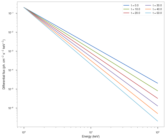
Now plot the synch. spectrum of the source at different times (you will need matplotlib for this)
[32]:
fig, ax = plt.subplots()
# Prepare 100 logarithmically distributed energies between 1 and 100 keV
energies = np.geomspace(1,100,100)

# Compute and plot the sync. spectrum every 10 s between 0 and 50 seconds

times = np.linspace(0,50,6)

my_model.time = 0.0

for tt in times:

    my_model.time = tt

    ax.loglog(energies, my_model.source_2.spectrum.synchrotron(energies),label='t = %s' % my_model.time.value)

ax.legend(loc=1,ncol=2)
ax.set_xlabel("Energy (keV)")
ax.set_ylabel(r"Differential flux (ph. cm$^{-2}$ s$^{-1}$ keV$^{-1}$)")
source_2
spectrum
synchrotron
time
source_2
spectrum
synchrotron
time
source_2
spectrum
synchrotron
time
source_2
spectrum
synchrotron
time
source_2
spectrum
synchrotron
time
source_2
spectrum
synchrotron
time
[32]:
Text(0, 0.5, 'Differential flux (ph. cm$^{-2}$ s$^{-1}$ keV$^{-1}$)')
[ ]: