Powerlaw Eflux
[3]:
# Parameters
func_name = "Powerlaw_Eflux"
wide_energy_range = True
x_scale = "log"
y_scale = "log"
linear_range = False
Description
[5]:
func.display()
- description: A power-law where the normalization is the energy flux defined between a and b
- formula: $ F~\frac{x}{piv}^{index} $
- parameters:
- F:
- value: 1e-05
- desc: Normalization (energy flux at the between a and b) erg /cm2 s
- min_value: 1e-30
- max_value: 1000.0
- unit:
- is_normalization: True
- delta: 0.1
- free: True
- piv:
- value: 1.0
- desc: Pivot value
- min_value: None
- max_value: None
- unit:
- is_normalization: False
- delta: 0.1
- free: False
- index:
- value: -2.0
- desc: Photon index
- min_value: -10.0
- max_value: 10.0
- unit:
- is_normalization: False
- delta: 0.2
- free: True
- a:
- value: 1.0
- desc: lower energy integral bound (keV)
- min_value: 0.0
- max_value: None
- unit:
- is_normalization: False
- delta: 0.1
- free: False
- b:
- value: 100.0
- desc: upper energy integral bound (keV)
- min_value: 0.0
- max_value: None
- unit:
- is_normalization: False
- delta: 10.0
- free: False
- F:
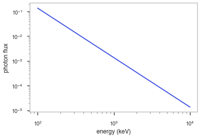
Shape
The shape of the function.
If this is not a photon model but a prior or linear function then ignore the units as these docs are auto-generated
[6]:
fig, ax = plt.subplots()


ax.plot(energy_grid, func(energy_grid), color=blue)

ax.set_xlabel("energy (keV)")
ax.set_ylabel("photon flux")
ax.set_xscale(x_scale)
ax.set_yscale(y_scale)
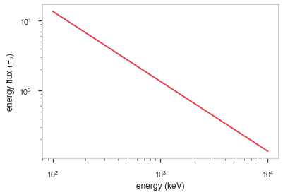
F\(_{\nu}\)
The F\(_{\nu}\) shape of the photon model if this is not a photon model, please ignore this auto-generated plot
[7]:
fig, ax = plt.subplots()

ax.plot(energy_grid, energy_grid * func(energy_grid), red)


ax.set_xlabel("energy (keV)")
ax.set_ylabel(r"energy flux (F$_{\nu}$)")
ax.set_xscale(x_scale)
ax.set_yscale(y_scale)
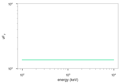
\(\nu\)F\(_{\nu}\)
The \(\nu\)F\(_{\nu}\) shape of the photon model if this is not a photon model, please ignore this auto-generated plot
[8]:
fig, ax = plt.subplots()

ax.plot(energy_grid, energy_grid**2 * func(energy_grid), color=green)


ax.set_xlabel("energy (keV)")
ax.set_ylabel(r"$\nu$F$_{\nu}$")
ax.set_xscale(x_scale)
ax.set_yscale(y_scale)