Truncated gaussian
[3]:
# Parameters
func_name = "Truncated_gaussian"
wide_energy_range = True
x_scale = "linear"
y_scale = "linear"
linear_range = True
Description
[5]:
func.display()
- description: A truncated Gaussian function defined on the interval between the lower_bound (a) and upper_bound (b)
- formula: $\begin{split}f(x;\mu,\sigma,a,b)=\frac{\frac{1}{\sigma} \phi\left( \frac{x-\mu}{\sigma} \right)}{\Phi\left( \frac{b-\mu}{\sigma} \right) - \Phi\left( \frac{a-\mu}{\sigma} \right)}\\\phi\left(z\right)=\frac{1}{\sqrt{2 \pi}}\exp\left(-\frac{1}{2}z^2\right)\\\Phi\left(z\right)=\frac{1}{2}\left(1+erf\left(\frac{z}{\sqrt(2)}\right)\right)\end{split}$
- parameters:
- F:
- value: 1.0
- desc: Integral between -inf and +inf. Fix this to 1 to obtain a Normal distribution
- min_value: None
- max_value: None
- unit:
- is_normalization: False
- delta: 0.1
- free: True
- mu:
- value: 0.0
- desc: Central value
- min_value: None
- max_value: None
- unit:
- is_normalization: False
- delta: 0.1
- free: True
- sigma:
- value: 1.0
- desc: standard deviation
- min_value: 1e-12
- max_value: None
- unit:
- is_normalization: False
- delta: 0.1
- free: True
- lower_bound:
- value: -1.0
- desc: lower bound of gaussian, setting to -np.inf results in half normal distribution
- min_value: None
- max_value: None
- unit:
- is_normalization: False
- delta: 0.1
- free: True
- upper_bound:
- value: 1.0
- desc: upper bound of gaussian setting to np.inf results in half normal distribution
- min_value: None
- max_value: None
- unit:
- is_normalization: False
- delta: 0.1
- free: True
- F:
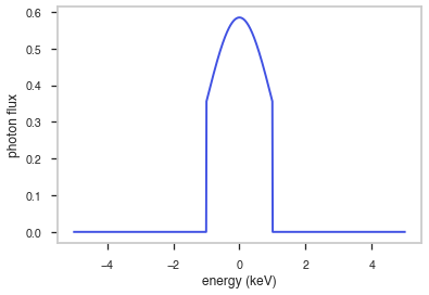
Shape
The shape of the function.
If this is not a photon model but a prior or linear function then ignore the units as these docs are auto-generated
[6]:
fig, ax = plt.subplots()


ax.plot(energy_grid, func(energy_grid), color=blue)

ax.set_xlabel("energy (keV)")
ax.set_ylabel("photon flux")
ax.set_xscale(x_scale)
ax.set_yscale(y_scale)
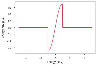
F\(_{\nu}\)
The F\(_{\nu}\) shape of the photon model if this is not a photon model, please ignore this auto-generated plot
[7]:
fig, ax = plt.subplots()

ax.plot(energy_grid, energy_grid * func(energy_grid), red)


ax.set_xlabel("energy (keV)")
ax.set_ylabel(r"energy flux (F$_{\nu}$)")
ax.set_xscale(x_scale)
ax.set_yscale(y_scale)
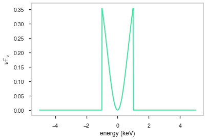
\(\nu\)F\(_{\nu}\)
The \(\nu\)F\(_{\nu}\) shape of the photon model if this is not a photon model, please ignore this auto-generated plot
[8]:
fig, ax = plt.subplots()

ax.plot(energy_grid, energy_grid**2 * func(energy_grid), color=green)


ax.set_xlabel("energy (keV)")
ax.set_ylabel(r"$\nu$F$_{\nu}$")
ax.set_xscale(x_scale)
ax.set_yscale(y_scale)