Band Calderone
[3]:
# Parameters
func_name = "Band_Calderone"
wide_energy_range = True
x_scale = "log"
y_scale = "log"
linear_range = False
Description
[5]:
func.display()
- description: The Band model from Band et al. 1993, implemented however in a way which reduces the covariances between the parameters (Calderone et al., MNRAS, 448, 403C, 2015)
- formula: $ \text{(Calderone et al., MNRAS, 448, 403C, 2015)} $
- parameters:
- alpha:
- value: -1.0
- desc: The index for x smaller than the x peak
- min_value: -10.0
- max_value: 10.0
- unit:
- is_normalization: False
- delta: 0.1
- free: True
- beta:
- value: -2.2
- desc: index for x greater than the x peak (only if opt=1, i.e., for the Band model)
- min_value: -7.0
- max_value: -1.0
- unit:
- is_normalization: False
- delta: 0.22000000000000003
- free: True
- xp:
- value: 200.0
- desc: position of the peak in the x*x*f(x) space (if x is energy, this is the nuFnu or SED space)
- min_value: 0.0
- max_value: None
- unit:
- is_normalization: False
- delta: 20.0
- free: True
- F:
- value: 1e-06
- desc: integral in the band defined by a and b
- min_value: None
- max_value: None
- unit:
- is_normalization: True
- delta: 1e-07
- free: True
- a:
- value: 1.0
- desc: lower limit of the band in which the integral will be computed
- min_value: 0.0
- max_value: None
- unit:
- is_normalization: False
- delta: 0.1
- free: False
- b:
- value: 10000.0
- desc: upper limit of the band in which the integral will be computed
- min_value: 0.0
- max_value: None
- unit:
- is_normalization: False
- delta: 1000.0
- free: False
- opt:
- value: 1.0
- desc: option to select the spectral model (0 corresponds to a cutoff power law, 1 to the Band model)
- min_value: 0.0
- max_value: 1.0
- unit:
- is_normalization: False
- delta: 0.1
- free: False
- alpha:
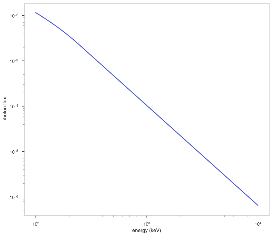
Shape
The shape of the function.
If this is not a photon model but a prior or linear function then ignore the units as these docs are auto-generated
[6]:
fig, ax = plt.subplots()


ax.plot(energy_grid, func(energy_grid), color=blue)

ax.set_xlabel("energy (keV)")
ax.set_ylabel("photon flux")
ax.set_xscale(x_scale)
ax.set_yscale(y_scale)
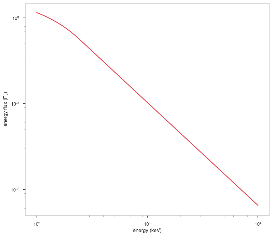
F\(_{\nu}\)
The F\(_{\nu}\) shape of the photon model if this is not a photon model, please ignore this auto-generated plot
[7]:
fig, ax = plt.subplots()

ax.plot(energy_grid, energy_grid * func(energy_grid), red)


ax.set_xlabel("energy (keV)")
ax.set_ylabel(r"energy flux (F$_{\nu}$)")
ax.set_xscale(x_scale)
ax.set_yscale(y_scale)
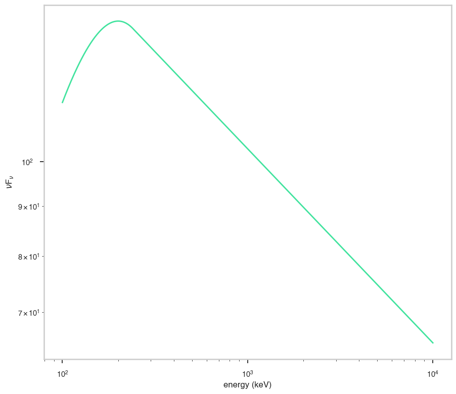
\(\nu\)F\(_{\nu}\)
The \(\nu\)F\(_{\nu}\) shape of the photon model if this is not a photon model, please ignore this auto-generated plot
[8]:
fig, ax = plt.subplots()

ax.plot(energy_grid, energy_grid**2 * func(energy_grid), color=green)


ax.set_xlabel("energy (keV)")
ax.set_ylabel(r"$\nu$F$_{\nu}$")
ax.set_xscale(x_scale)
ax.set_yscale(y_scale)