Log parabola
[3]:
# Parameters
func_name = "Log_parabola"
wide_energy_range = True
x_scale = "log"
y_scale = "log"
linear_range = False
Description
[5]:
func.display()
- description: A log-parabolic function. NOTE that we use the high-energy convention of using the natural log in place of the base-10 logarithm. This means that beta is a factor 1 / log10(e) larger than what returned by those software using the other convention.
- formula: $ K \left( \frac{x}{piv} \right)^{\alpha -\beta \log{\left( \frac{x}{piv} \right)}} $
- parameters:
- K:
- value: 1.0
- desc: Normalization
- min_value: 1e-30
- max_value: 100000.0
- unit:
- is_normalization: True
- delta: 0.1
- free: True
- piv:
- value: 1.0
- desc: Pivot (keep this fixed)
- min_value: None
- max_value: None
- unit:
- is_normalization: False
- delta: 0.1
- free: False
- alpha:
- value: -2.0
- desc: index
- min_value: None
- max_value: None
- unit:
- is_normalization: False
- delta: 0.2
- free: True
- beta:
- value: 1.0
- desc: curvature (positive is concave, negative is convex)
- min_value: None
- max_value: None
- unit:
- is_normalization: False
- delta: 0.1
- free: True
- K:
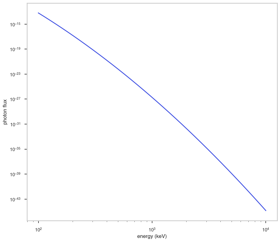
Shape
The shape of the function.
If this is not a photon model but a prior or linear function then ignore the units as these docs are auto-generated
[6]:
fig, ax = plt.subplots()


ax.plot(energy_grid, func(energy_grid), color=blue)

ax.set_xlabel("energy (keV)")
ax.set_ylabel("photon flux")
ax.set_xscale(x_scale)
ax.set_yscale(y_scale)
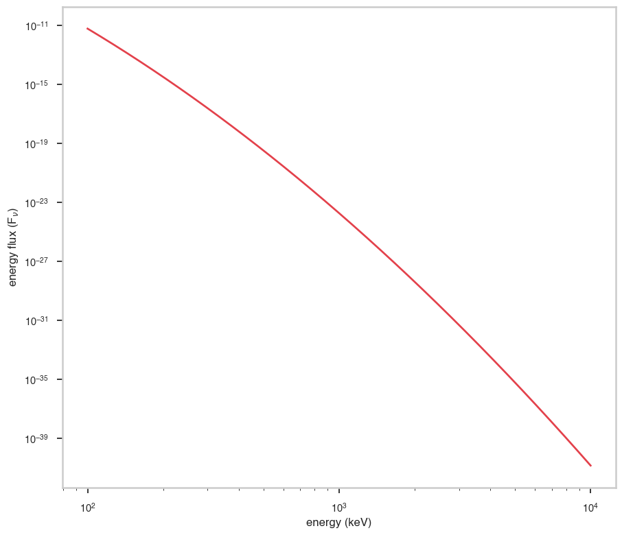
F\(_{\nu}\)
The F\(_{\nu}\) shape of the photon model if this is not a photon model, please ignore this auto-generated plot
[7]:
fig, ax = plt.subplots()

ax.plot(energy_grid, energy_grid * func(energy_grid), red)


ax.set_xlabel("energy (keV)")
ax.set_ylabel(r"energy flux (F$_{\nu}$)")
ax.set_xscale(x_scale)
ax.set_yscale(y_scale)
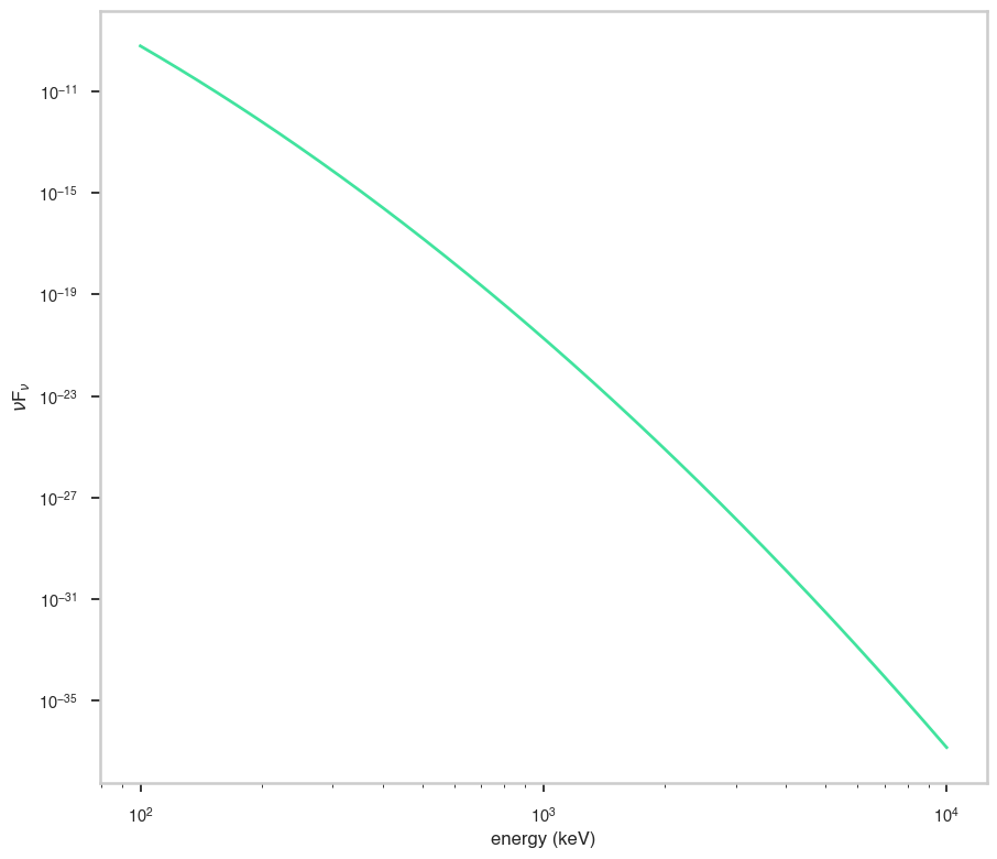
\(\nu\)F\(_{\nu}\)
The \(\nu\)F\(_{\nu}\) shape of the photon model if this is not a photon model, please ignore this auto-generated plot
[8]:
fig, ax = plt.subplots()

ax.plot(energy_grid, energy_grid**2 * func(energy_grid), color=green)


ax.set_xlabel("energy (keV)")
ax.set_ylabel(r"$\nu$F$_{\nu}$")
ax.set_xscale(x_scale)
ax.set_yscale(y_scale)