Uniform prior
[3]:
# Parameters
func_name = "Uniform_prior"
wide_energy_range = True
x_scale = "linear"
y_scale = "linear"
linear_range = True
Description
[5]:
func.display()
- description: A function which is constant on the interval lower_bound - upper_bound and 0 outside the interval. The extremes of the interval are counted as part of the interval.
- formula: $ f(x)=\begin{cases}0 & x < \text{lower_bound} \\\text{value} & \text{lower_bound} \le x \le \text{upper_bound} \\ 0 & x > \text{upper_bound} \end{cases}$
- parameters:
- lower_bound:
- value: 0.0
- desc: Lower bound for the interval
- min_value: -inf
- max_value: inf
- unit:
- is_normalization: False
- delta: 0.1
- free: True
- upper_bound:
- value: 1.0
- desc: Upper bound for the interval
- min_value: -inf
- max_value: inf
- unit:
- is_normalization: False
- delta: 0.1
- free: True
- value:
- value: 1.0
- desc: Value in the interval
- min_value: None
- max_value: None
- unit:
- is_normalization: False
- delta: 0.1
- free: True
- lower_bound:
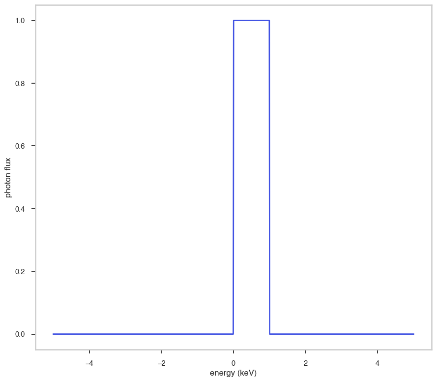
Shape
The shape of the function.
If this is not a photon model but a prior or linear function then ignore the units as these docs are auto-generated
[6]:
fig, ax = plt.subplots()


ax.plot(energy_grid, func(energy_grid), color=blue)

ax.set_xlabel("energy (keV)")
ax.set_ylabel("photon flux")
ax.set_xscale(x_scale)
ax.set_yscale(y_scale)
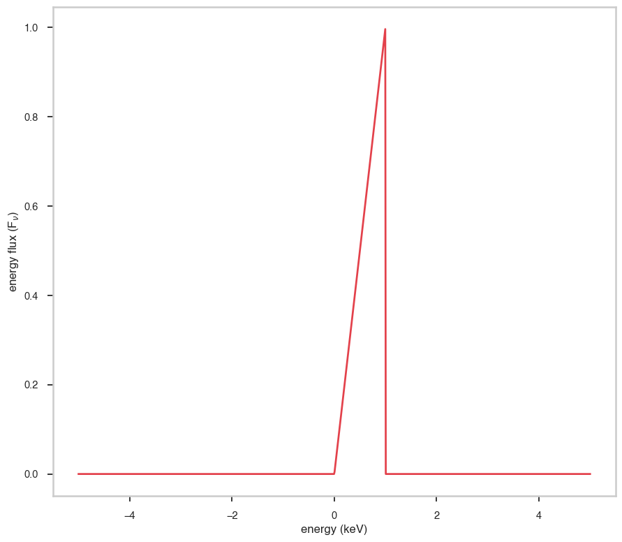
F\(_{\nu}\)
The F\(_{\nu}\) shape of the photon model if this is not a photon model, please ignore this auto-generated plot
[7]:
fig, ax = plt.subplots()

ax.plot(energy_grid, energy_grid * func(energy_grid), red)


ax.set_xlabel("energy (keV)")
ax.set_ylabel(r"energy flux (F$_{\nu}$)")
ax.set_xscale(x_scale)
ax.set_yscale(y_scale)
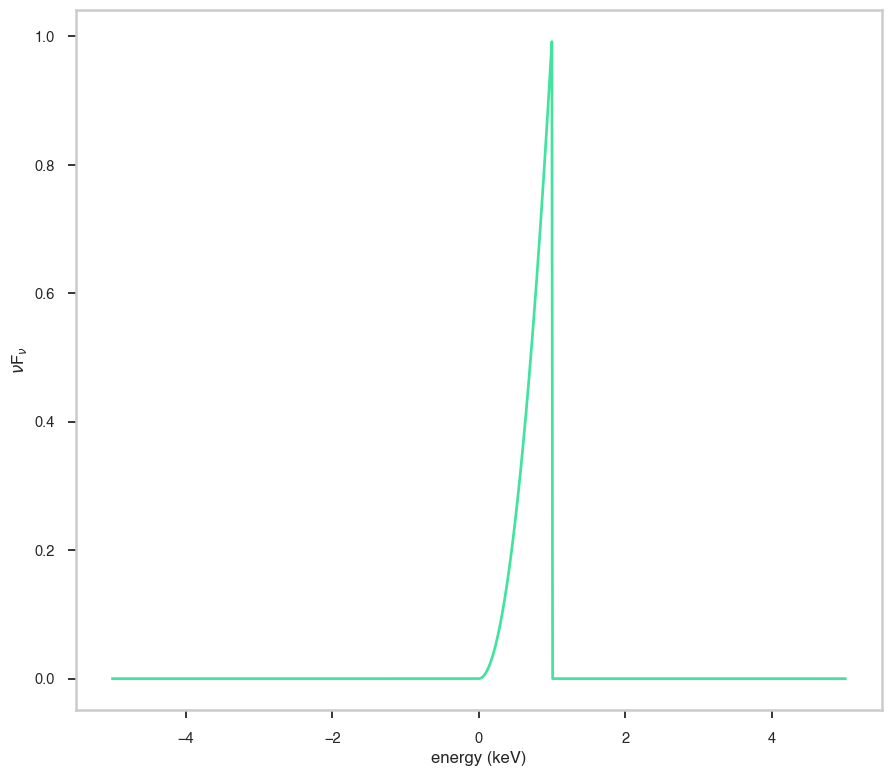
\(\nu\)F\(_{\nu}\)
The \(\nu\)F\(_{\nu}\) shape of the photon model if this is not a photon model, please ignore this auto-generated plot
[8]:
fig, ax = plt.subplots()

ax.plot(energy_grid, energy_grid**2 * func(energy_grid), color=green)


ax.set_xlabel("energy (keV)")
ax.set_ylabel(r"$\nu$F$_{\nu}$")
ax.set_xscale(x_scale)
ax.set_yscale(y_scale)